algebra 1 final exam study guide

Core Algebraic Concepts

Key topics for the Algebra 1 final include understanding associative‚ commutative‚ and distributive laws‚ solving linear equations‚ simplifying expressions with positive exponents‚ and applying properties to factor polynomials. Practice.

Basic Properties of Operations

The Associative‚ Commutative‚ Distributive‚ Identity‚ and Inverse properties are the foundation of algebraic manipulation. The Associative Property states that when adding or multiplying three or more numbers‚ the grouping does not affect the result: (a + b) + c = a + (b + c) and (a × b) × c = a × (b × c). The Commutative Property allows the order of addition or multiplication to be changed: a + b = b + a and a × b = b × a. The Distributive Property links addition and multiplication: a × (b + c) = a × b + a × c. Identity elements keep a number unchanged: a + 0 = a and a × 1 = a. Inverse elements cancel each other: a + (–a) = 0 and a × (1/a) = 1 for a ≠ 0. Mastery of these properties enables simplification‚ equation solving‚ and factoring‚ all critical for the final exam. Practice identifying and applying each property in diverse problems to build fluency and confidence. Mastery of these concepts is essential for success on the final exam‚ and consistent practice will reinforce understanding. By applying these properties systematically‚ students can simplify complex expressions‚ solve equations efficiently‚ and approach problems with confidence. Consistent review of these properties will build a strong algebra foundation and prepare students for higher-level math courses. This guide consolidates concepts for exam readiness!

Solving Linear Equations

Linear equations involve one variable and can be solved by isolating the variable. Begin by simplifying each side‚ combining like terms‚ and moving all variable terms to one side while constants go to the opposite side.

Use the inverse operations: addition/subtraction to eliminate constants‚ and multiplication/division to isolate the variable. For example‚ solving 5x – (x + 3) = 5 requires distributing the negative sign‚ yielding 5x – x – 3 = 5‚ then combining like terms to get 4x – 3 = 5‚ adding 3 to both sides‚ and finally dividing by 4 to find x = 2.

Check your solution by substituting back into the original equation to ensure both sides are equal. Mistakes often arise from incorrect sign distribution or arithmetic errors. Practice with problems that include parentheses‚ fractions‚ and negative coefficients.

When encountering equations with fractions‚ multiply every term by the least common denominator to clear fractions before simplifying. For inequalities‚ remember that multiplying or dividing by a negative reverses the inequality sign. Always verify solutions by plugging them back into the equation or inequality!

Key strategies: always keep the variable on one side‚ simplify before solving‚ and double‑check each step. Mastering these steps will build confidence for the final exam.

Graphing and Functions

Master graphing linear functions by plotting points‚ finding intercepts‚ and using slope–intercept form y=mx+b. Understand how slope indicates steepness and direction while they‑intercept shows where the line crosses the y‑axis. Practice converting equations to graphs.

Graphing Linear Functions

To graph a linear function y = mx + b‚ identify the slope m and y‑intercept b. The y‑intercept is the point (0‚ b) where the line crosses the y‑axis. The slope m represents the change in y per unit change in x; it can be expressed as rise over run. Use two points to plot the line: start at (0‚ b)‚ then move right by one unit and up by m units (if m>or down by |m| units (if m<0). Alternatively‚ if a second point is given‚ compute the slope as (y₂–y₁)/(x₂–x₁) and use it to find a third point. Once two points are on the graph‚ draw a straight line through them extending in both directions. Check accuracy by substituting a test x‑value into the equation and verifying the plotted y‑coordinate. For negative slopes‚ the line descends from left to right; for positive slopes‚ it ascends. The slope sign also indicates whether the function is increasing or decreasing. Remember that vertical lines (undefined slope) cannot be expressed in slope‑intercept form.

When sketching‚ label the axes‚ choose a suitable scale‚ and plot points accurately. A line with a positive slope rises from left to right‚ while a negative slope falls. The y‑intercept gives a starting point; the slope tells how steep the line is. Practice drawing several lines to build confidence.

Finally‚ double‑check plotted points to ensure the line matches the equation now!!

Interpreting Slope and Intercept

When you read a linear equation in slope‑intercept form‚ y = mx + b‚ the slope m tells you how steep the line rises or falls for each unit increase in x. A positive m means the line climbs upward; a negative m means it descends. The absolute value of m indicates steepness: |m| > 1 gives a steep line‚ |m| < 1 gives a shallow line‚ and m = 0 gives a horizontal line. The y‑intercept b is the point where the line crosses the y‑axis‚ i.e.‚ the value of y when x = 0. If b is positive‚ the line starts above the origin; if b is negative‚ it starts below. The x‑intercept is found by setting y = 0 and solving for x‚ giving the point where the line crosses the x‑axis. In graphing‚ the slope also determines the ratio of rise over run‚ so a slope of 3/2 means the line rises 3 units for every 2 units moved right. Recognizing these relationships lets you sketch accurate graphs‚ predict values‚ and solve real‑world problems involving rates and trends.

When graphing‚ remember that a slope of zero produces a flat line‚ while a vertical line has an undefined slope. The y‑intercept can be found by plugging x = 0 into the equation‚ and the x‑intercept by setting y = 0. These intercepts help locate key points on the graph‚ enabling quick checks of accuracy.

Practice!

Systems and Inequalities

Master linear systems by substitution‚ elimination‚ and graphing. Practice inequalities: write solution intervals‚ shade on number lines‚ and solve compound forms. Review critical point tests and boundary checks for accuracy. Keep up!!!

Solving Systems of Equations

Mastering systems of linear equations is essential for the Algebra 1 final. Students should be comfortable with three primary techniques: substitution‚ elimination‚ and graphing. In substitution‚ solve one equation for a variable‚ then substitute that expression into the other equation to reduce the system to a single variable. Elimination‚ also known as the addition method‚ involves adding or subtracting equations after scaling them so that one variable cancels out‚ leaving a solvable equation for the remaining variable. Graphing requires plotting each line on the same coordinate plane; the intersection point gives the solution pair. For larger systems‚ matrix methods or using the determinant (Cramer’s rule) can be efficient‚ but the exam typically focuses on the first three. Practice by converting word problems into equations‚ simplifying‚ and applying the chosen method systematically. Pay attention to domain restrictions and check solutions by substitution back into the original equations. Consistent practice with varied coefficient sizes‚ including fractions and negative numbers‚ builds confidence and speeds up problem‑solving during the test. Remember‚ the key to mastering systems is practice: solve a variety of problems‚ check each answer by plugging back into both equations‚ and review any mistakes to reinforce the underlying concepts and strategies well.!

Inequality Graphing

To graph a linear inequality‚ rewrite it in slope‑intercept form y = mx + b. If the inequality is <‚ ≤‚ >‚ or ≥‚ draw the boundary line accordingly: a solid line for ≤ or ≥‚ a dashed line for < or >. Shade the half‑plane that satisfies the inequality. Use a test point—usually (0‚0)—to decide which side to shade. For example‚ y > 2x + 3: the line y = 2x + 3 is dashed; test (0‚0) gives 0 > 3? No‚ so shade above the line. If the inequality is ≥‚ the boundary is solid and the shading includes the line. For systems of inequalities‚ shade each region and find the intersection of all shaded areas; that intersection is the solution set.

When dealing with non‑linear inequalities‚ such as y ≤ x²‚ plot the curve y = x² first‚ then shade below the parabola for ≤ or above for ≥. For inequalities involving fractions or absolute values‚ simplify before graphing. Check boundary points by substituting them back into the inequality to confirm whether they belong to the solution set. In a test setting‚ sketching and labeling can save time‚ but double‑checking the shaded region against a test point ensures accuracy. Check endpoints for inclusivity. Test!

Advanced Topics

Polynomials: factor by grouping‚ use zero‑product property. Exponents: rewrite negative exponents as reciprocals‚ apply power rules. Radicals: rationalize denominators‚ combine like radicals. Practice with sample problems from the PDF source.!!!

Polynomials and Factoring

Polynomials are algebraic expressions composed of variables and coefficients combined with addition‚ subtraction‚ multiplication‚ and exponentiation. Mastery of factoring is essential for solving equations‚ simplifying expressions‚ and graphing. Begin by extracting the greatest common factor (GCF). For example‚ in 6x³−12x²+18x‚ the GCF is 6x‚ yielding 6x(x²−2x+3). Next‚ factor quadratic trinomials of the form ax²+bx+c. Use the AC method or trial‑and‑error to find two numbers that multiply to a·c and add to b. For instance‚ x²+5x+6 factors to (x+2)(x+3). Recognize special products: difference of squares a²−b²=(a−b)(a+b); perfect square trinomials a²+2ab+b²=(a+b)²; and sum/difference of cubes a³±b³=(a±b)(a²∓ab+b²). When the quadratic is not factorable over the integers‚ apply the quadratic formula x=[−b±√(b²−4ac)]/(2a). Practice factoring polynomials of higher degree by grouping: x³−3x²+4x−12 can be grouped as (x³−3x²)+(4x−12)=x²(x−3)+4(x−3)=(x²+4)(x−3). Always verify by expanding the factored form. A solid grasp of these techniques will streamline solving equations‚ simplifying rational expressions‚ and preparing for the final exam. Students should also practice factoring by inspection and using the factor theorem to identify roots‚ strengthening algebraic fluency.!! Remember to test factor by substitution.

Exponents and Radicals

Mastering exponents and radicals is essential for the Algebra 1 final. Begin by recalling the laws of exponents: product rule (a^m·a^n = a^(m+n))‚ quotient rule (a^m/a^n = a^(m−n))‚ power rule ((a^m)^n = a^(mn))‚ and zero‑exponent rule (a^0 = 1). When encountering negative exponents‚ rewrite them as reciprocals: a^(−n) = 1/a^n. For example‚ the question “Which shows the expression below written with positive exponents? 3a( ) −4 b” requires converting 3a^(−4)b to 3a^4b⁻¹‚ then simplifying to a positive exponent form. Similarly‚ “Which shows the expression below written with positive exponents? 2d( ) 4 3d( ) 2” tests the ability to move negative exponents to the denominator. Radical notation is the inverse of exponentiation: √[n]{a} = a^(1/n). Practice converting between radical and fractional‑exponent forms‚ such as √[3]{x^2} = x^(2/3). When simplifying expressions that mix exponents and radicals‚ apply the product rule first‚ reduce fractional exponents When instance‚ simplifying 2c − 7c 8c involves factoring c and using the distributive property‚ as shown in the provided solution steps. Understanding these principles will allow you to solve problems like “What is the reciprocal of −47?” (answer: −1/47) and to correctly rewrite expressions with negative exponents. Consistent practice with these rules ensures accuracy on the exam.

Exam Strategies

Use timed practice tests‚ review key algebraic rules‚ prioritize problem types‚ skip tough questions‚ then return‚ check work‚ and manage time by allocating minutes per section. Stay calm‚ read carefully‚ and apply shortcuts wisely. Keep calm.

Time Management

Effective pacing is essential for the Algebra 1 final. Allocate a fixed time per question—typically 1–2 minutes for straightforward problems and 3–5 minutes for multi‑step items. Use a timer or stopwatch to stay on track. Begin with the easiest questions to secure quick points‚ then tackle harder ones. If you’re stuck‚ mark the problem‚ move on‚ and return if time allows. Keep a running tally of points earned versus time spent to gauge efficiency. Practice timed drills with past‑exam questions to build speed and confidence. Remember to leave a few minutes at the end for review and double‑checking calculations‚ especially for algebraic expressions involving exponents and factoring. Consistent practice improves both accuracy and speed‚ ensuring you can handle the full breadth of topics on test day.

During the exam‚ if a question impossible‚ skip it and return later to avoid time. After the test‚ review unanswered items to learn from mistakes and improve performance.

Resources and Practice

Utilize free online practice sets‚ review checklists‚ and sample exams from reputable sites. Focus on timed drills‚ concept quizzes‚ and peer discussion forums to reinforce algebraic skills before the final!!! Practice daily for mastery.

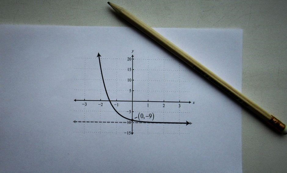
Review Checklist

• Associative‚ commutative‚ and distributive properties.
• Solve linear equations and inequalities.
• Simplify expressions with positive exponents.
• Factor quadratics and higher‑degree polynomials.
• Graph linear functions and interpret slope and intercept.
• Use substitution and elimination for systems of equations.
• Apply exponent rules and radical simplification.
• Check solutions for common algebraic errors.
• Practice timed problem sets.
• Review key formulas and identities.

Lorem ipsum dolor sit amet‚ consectetur adipiscing elit. Sed do eiusmod tempor incididunt ut labore et dolore magna aliqua. Ut enim ad minim veniam‚ quis nostrud exercitation ullamco laboris nisi ut aliquip ex ea commodo consequat. Duis aute irure dolor in reprehenderit in voluptate velit esse cillum dolore eu fugiat nulla pariatur. Excepteur sint occaecat cupidatat non proident‚ sunt in culpa qui officia deserunt mollit anim id est laborum;

Praesent volutpat nisl eget dignissim‚ sed tempor risus. Integer ac massa et odio faucibus. Vestibulum ante ipsum primis in faucibus orci luctus et ultrices posuere cubilia curae; Sed vitae justo at nisl convallis.

Cras at mauris non lorem tristique volutpat. Sed at massa vitae orci consectetur. Donec vel libero at justo lorem! .. ok

Practice Problem Sets

Below are targeted practice problems designed to reinforce the core concepts you’ll encounter on the Algebra 1 final. Work through each item‚ then check your answer against the provided solutions. These problems cover equation solving‚ factoring‚ exponents‚ radicals‚ and graph interpretation.

• Solve for x: 2(x + 3) – 4 = 10.
• Factor completely: x² – 9.
• Simplify: (4a³b²) ÷ (2a b).
• Write the expression 5a⁻²b³ with positive exponents.
• Find the slope and y‑intercept of y = –3x + 7.
• Solve the system: {3x + 2y = 12‚ x – y = 4}.
• Determine the domain of f(x) = √(x – 5).
• Expand: (2x – 3)(x + 4).
• Solve for y: y / (2y + 1) = 3.
• Identify the property used: a(b + c) = ab + ac.

After completing the set‚ review the solutions below and reflect on any patterns in mistakes. Consistent practice is the key to mastering Algebra 1.

Tip: When working with radicals‚ rationalize denominators and check for extraneous solutions after squaring both sides. For inequalities‚ remember that multiplying or dividing by a negative number reverses the inequality sign. Practice these steps until they become second nature.

Remember to check each step‚ keep work organized‚ use back‑of‑the‑envelope estimates to verify reasonableness of answers.